Imagine you’re in a pool, and you’re trying to push a float. Right at the surface of the float, the water is completely still. It’s stuck to the float. As you move away from the surface, the water starts to move faster and faster until it reaches the speed of the main current. This thin layer of water, where the speed changes from zero to the full current speed, is called the Boundary layer.
Now, imagine we need to build a virtual version of this float and the water around it on a computer to see how it will behave. We’d use a method called Computational Fluid Dynamics (CFD). To do this, we break the space around the float into tiny little boxes or a mesh.
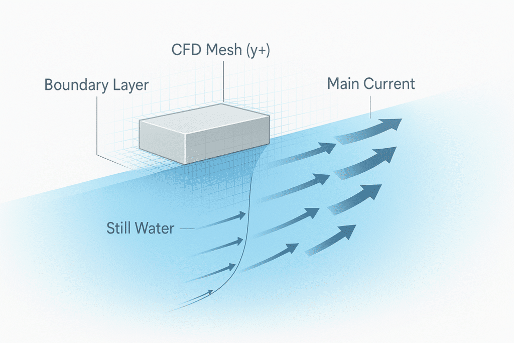
y+ is simply a number that tells us how big the first layer of these little boxes is, right next to the float’s surface. Think of it as a quality check for our virtual model. It helps us know if our tiny boxes are the right size to accurately capture what’s happening in that all-important boundary layer.
Table of Contents
Why is y+ Important?
Getting the y+ value right is critical for a couple of reasons:
- Accuracy: The boundary layer is where important things happen, like friction and heat transfer. If our virtual boxes (mesh) are too big in this area, we’ll miss the details. The results for things like drag and lift on our object will be wrong.
- Computational Cost: Making the boxes too small everywhere will give us accurate results but will require a massive amount of computing power and time. It’s like trying to count every single grain of sand on a beach when you only need a rough estimate. y+ helps us find the sweet spot, where the boxes are just the right size in the critical boundary layer, and we can use bigger boxes everywhere else to save time and money.
What’s a Good y+ Value?
The “right” value for y+ depends on what we’re trying to measure and the type of virtual model (turbulence model) we’re using.
- Low y+ (around 1): We use this when we need extremely high accuracy, especially for friction and heat transfer. This requires very tiny boxes close to the surface, which is computationally expensive but provides the most detailed results.
- High y+ (around 30-300): This is used when we don’t need to resolve the boundary layer in detail. We’re essentially using a shortcut formula to estimate what happens in that layer. This is much faster and less expensive computationally, but less accurate for things happening right at the surface.
In short, y+ is a key metric in CFD that helps engineers make sure their computer simulations are both Accurate and Efficient by controlling the size of the mesh near the surface of an object. It’s a simple number with a big impact on the quality of the simulation.
y+ in Technical
y+ is a dimensionless number used in Computational Fluid Dynamics (CFD) that represents the distance of the first mesh cell from a solid wall in a fluid simulation. It helps engineers determine if the mesh resolution near a surface is fine enough to accurately capture the fluid’s behavior, particularly the boundary layer, which is the thin region of fluid where velocity changes from zero at the wall to the free-stream velocity. Choosing the right y+ value is critical for ensuring simulation accuracy and efficiency.
The Technical Details: What y+ Really Means
To fully understand y+, let’s break down its components. The formula for y+ is:
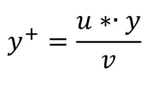
- y: The physical distance from the wall to the center of the first mesh cell.
- ν: The kinematic viscosity of the fluid, which is its resistance to flow. Think of it as how “sticky” the fluid is. Water has a low viscosity, while honey has a high one.
- u: The friction velocity, a concept that might not be intuitive. It’s a scaling factor for velocity related to the shear stress at the wall. It’s not a real velocity but a mathematical construct that helps us normalize the flow.
In essence, y+ takes a physical distance (y) and makes it dimensionless by scaling it with the fluid’s properties (ν) and the local flow conditions (u∗). This allows us to compare the grid resolution near the wall in different simulations and with different fluids.
The Boundary Layer and Its Regions
The boundary layer is not a uniform region; it’s made of distinct layers, each with its own characteristics. In a turbulent flow, we can identify three primary regions based on their y+ values:
- Viscous Sub-layer (0<y+<6): This region is right next to the wall. The flow is dominated by viscous forces, and it behaves almost like a laminar (smooth, non-chaotic) flow. The relationship between the non-dimensional velocity (u+) and y+ is linear: u+=y+.
- Transition or Buffer Layer (6<y+<30): In this region, the flow begins to transition from a viscous-dominated regime to a turbulent one. Both viscous and turbulent effects are significant.
- Log-law Region (30<y+<1000): Here, the flow is fully turbulent. The velocity profile follows a logarithmic relationship: u+=κln(y+)+A, where κ (Karman’s constant) is approximately 0.4 and A is a model constant (around 5.5). This is where turbulent diffusion becomes prominent.
The Role of y+ in Turbulence Modeling
In CFD, we use different turbulence models to simulate complex flows. These models have specific requirements for the y+ value of the mesh at the wall.
High-Reynolds Turbulence Models
These models (e.g., k-epsilon, k-omega) are based on the assumption that the first mesh cell is located in the log-law region of the boundary layer. They use a “wall function” to bridge the gap between the wall and the first mesh cell, effectively bypassing the need to resolve the viscous sub-layer.
- Recommended y+: The mesh should be generated so that y+ is in the range of 30 to 1000.
- How They Work: The model automatically switches its behavior based on the calculated y+ value. If y+>11.6 (the intersection point of the viscous sub-layer and log-law lines), it applies a log-law condition. If y+<11.6, it applies a non-slip (laminar-like) condition.
Low-Reynolds Turbulence Models
These models (e.g., low-Reynolds number k-epsilon) are specifically designed to resolve the flow right down to the wall, including the viscous sub-layer. They don’t rely on wall functions and are more computationally expensive but offer higher accuracy for applications where wall effects (like heat transfer and skin friction drag) are critical.
- Recommended y+: For the best accuracy, the mesh should be generated so that y+ is less than 1.0.
- How They Work: They use an “adaptive wall function” or exact boundary conditions to resolve the flow near the wall without switching based on y+ value. The objective is to capture the flow physics in the y+<30 region.
FAQ: Common Questions About y+
Why not always use a very small y+ for perfect accuracy?
While a very small y+ (around 1) with a low-Reynolds model offers high accuracy, it dramatically increases the number of mesh cells required, leading to significantly longer simulation times and higher computational costs. For many engineering applications, the faster, less expensive high-Reynolds models with a larger y+ are sufficient.
How do engineers control the y+ value in their simulations?
Engineers control y+ by adjusting the size of the first mesh cell adjacent to the wall. They can either use a trial-and-error approach or, more commonly, use an estimation formula before meshing to calculate the required first cell height based on the expected flow conditions (Reynolds number).
Can I have a mixed y+ mesh in my simulation?
Yes, it’s possible, especially in complex geometries. However, it requires careful implementation and is generally not recommended as it can lead to inaccuracies and convergence issues. It’s best practice to choose a single y+ strategy (high- or low-Reynolds) and apply it consistently to all wall surfaces.
Summary
The article explains y+, a crucial concept in Computational Fluid Dynamics (CFD), to a non-technical audience. It begins by using a simple analogy of a float in a pool to describe the boundary layer—the thin layer of fluid where velocity changes from zero to the free-stream velocity. The article defines y+ as a dimensionless number that acts as a quality check for the computational mesh, specifically telling us how large the first layer of mesh cells is, right next to a solid surface. This number is critical for balancing a simulation’s accuracy and computational cost.
The article then dives into the technical details, providing the formula for y+ and explaining the three distinct regions of a turbulent boundary layer: the viscous sub-layer (y+<6), the transition layer (6<y+<30), and the log-law region (30<y+<1000). It clarifies that different turbulence models have specific requirements for y+. High-Reynolds models are computationally cheaper and use a high y+ value (30-1000), while Low-Reynolds models require a very low y+ (ideally < 1) for higher accuracy, making them more expensive. Finally, the article provides an FAQ section that addresses common questions, reinforcing that engineers control y+ by adjusting the mesh size and that consistency is key for accurate results.
Key Takeaways
- What is y+? It’s a dimensionless number in CFD that represents the size of the first mesh cell off a wall. It’s a critical quality check for a simulation’s mesh.
- Why is it important? It’s a trade-off between accuracy (capturing the boundary layer details) and computational cost (running the simulation efficiently).
- The Boundary Layer has distinct regions. In turbulent flow, the boundary layer is not uniform. It consists of a viscous sub-layer, a transition layer, and a log-law region.
- The “right” y+ value depends on the turbulence model.
- High-Reynolds models (e.g., k-epsilon) use a wall function and need a high y+ (30-1000) because they don’t resolve the details right at the wall.
- Low-Reynolds models need a very low y+ (ideally < 1) to capture the viscous sub-layer accurately, making them more computationally expensive but also more precise for certain applications.
- Engineers control y+ by carefully setting the size of the mesh elements nearest to the wall.
- Consistency is key. It’s best practice to use a consistent y+ strategy across all wall surfaces in a simulation to avoid inaccuracies.