Smart Thermostat Simulation in scFLOW | Automate HVAC Control with Scripting

When designing HVAC systems, it’s important to simulate real-world automatic temperature regulation. This tutorial shows how to use scFLOW’s scripting capabilities to create a simple thermostatic control system that adjusts air supply temperature in response to feedback from a monitoring point. By integrating logic-based automation directly into your CFD model, you can create more realistic and efficient HVAC simulations.

---

🎯 Objective

We aim to simulate a scenario where the inlet air temperature is automatically adjusted to maintain a target temperature at a specific downstream location. This mirrors how a real-world thermostat maintains comfort conditions by regulating HVAC output.

🛠 Simulation Conditions

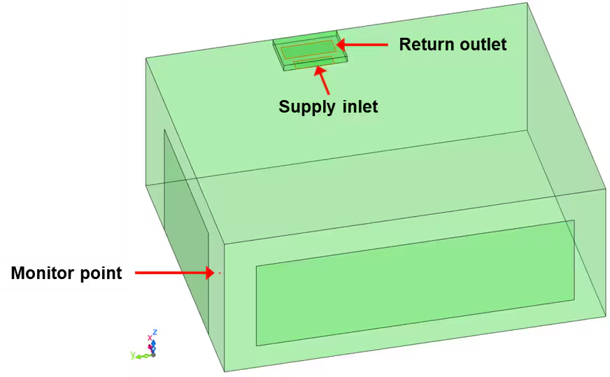
We’ll simulate airflow within a room and define the following conditions:

• Room Dimensions: 5.0 × 6.0 × 2.4 meters
• Initial Room and Air Supply Temperature: 20.0°C
• Window Conditions:
  • Fixed temperature: 36.0°C
  • Heat transfer coefficient: 20 W/(m²·K)
• Air Supply and Return Flow Rate: 9.5 m³/min
• Thermostat Point: (0.5, 5.95, 1.5) m
• Cooling Logic:
  • If temperature at monitor point > 21°C → Air supply = 10°C
  • If temperature < 20°C → Air supply = 20°C

---

🧩 Step-by-Step Setup in scFLOW

1. Open Base Model

Start with the provided room.pph model in scFLOW. Confirm the presence of sheet parts:

• [Supply], [Return], [Window_x], [Window_y]
• A monitoring point labeled [Point_1]
• Predefined transient settings: 2400 steps, 0.5s time step

2. Define Supply Temperature via Formatted Script

• Go to the Flow Boundary screen in Condition Wizard
• Double-click on [Flux] condition on the [Supply] surface
• In [Inflow Temperature], select Formatted Script

Code: [usr_bcflowval] Setting Function

var line = [];
var msg, tmp;

// Read thermostat coordinates from input
usf_getline(line, 200);
tmp = line[0].split(' ');
xyz_pt[0] = parseFloat(tmp[0]);
xyz_pt[1] = parseFloat(tmp[1]);
xyz_pt[2] = parseFloat(tmp[2]);
usf_sout("===== Thermostat point: " + xyz_pt);

// Read standard and cooling temperatures
usf_getline(line, 200);
tmp = line[0].split(' ');
T_standard = parseFloat(tmp[0]);
T_cool = parseFloat(tmp[1]);
usf_sout("===== Standard and cooling temperatures: " + T_standard + ", " + T_cool);

// Read thresholds for turning cooling on/off
usf_getline(line, 200);
tmp = line[0].split(' ');
T_turn_on = parseFloat(tmp[0]);
T_turn_off = parseFloat(tmp[1]);
usf_sout("===== Cooling ON/OFF thresholds: " + T_turn_on + ", " + T_turn_off);

Explanation: This block reads the thermostat control parameters from the SPH input file, such as the point coordinates and temperature thresholds, and stores them in global variables.

3. Set Function Name and Return Value

• In [Function Name] select use_bcflowval

return T_in;

Explanation: This returns the dynamically updated air supply temperature, which is controlled via logic in the timing functions.

4. Define Global Variables in Script Panel

var xyz_pt = [];       // Coordinates of monitor point
var ie_pt = [];        // Element index containing the monitor point
var T_pt;              // Temperature at monitor point
var T_standard, T_cool; // Standard and cooled air temperatures
var T_turn_on, T_turn_off; // Thresholds for switching cooling on/off
var T_in;              // Final input temperature to be used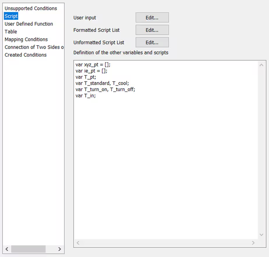

Explanation: These variables will be used across functions to store thermostat logic values and state.

5. Set [usu_init] Function

var rank_pt = [];
usf_find_xyz_ie(xyz_pt, ie_pt, rank_pt);
if(rank_pt[0] == -1){
  usf_stop("===== Error: Thermostat point not found in domain");
}

Explanation: This function runs at simulation startup to identify which mesh element contains the monitor point. If the point isn’t in the mesh, the simulation is halted.

6. Set [usu_cycle_start] Logic

var tmp_T = [];
var ncycle;

tmp_T[0] = -999;
if(ie_pt[0] >= 0){
  usf_get_elem_fdata(ie_pt[0], $IVAR_TEMP, tmp_T); // Get temperature
}
T_pt = mpi_max(tmp_T[0]); // Assign temp using parallel-safe max value
usf_sout("===== Temperature at monitor point: " + T_pt);

ncycle = usf_ncyc();
if(ncycle == 1){
  T_in = T_standard; // Set to default on first step
}else if(T_pt > T_turn_on){
  T_in = T_cool;
}else if(T_pt < T_turn_off){
  T_in = T_standard;
}

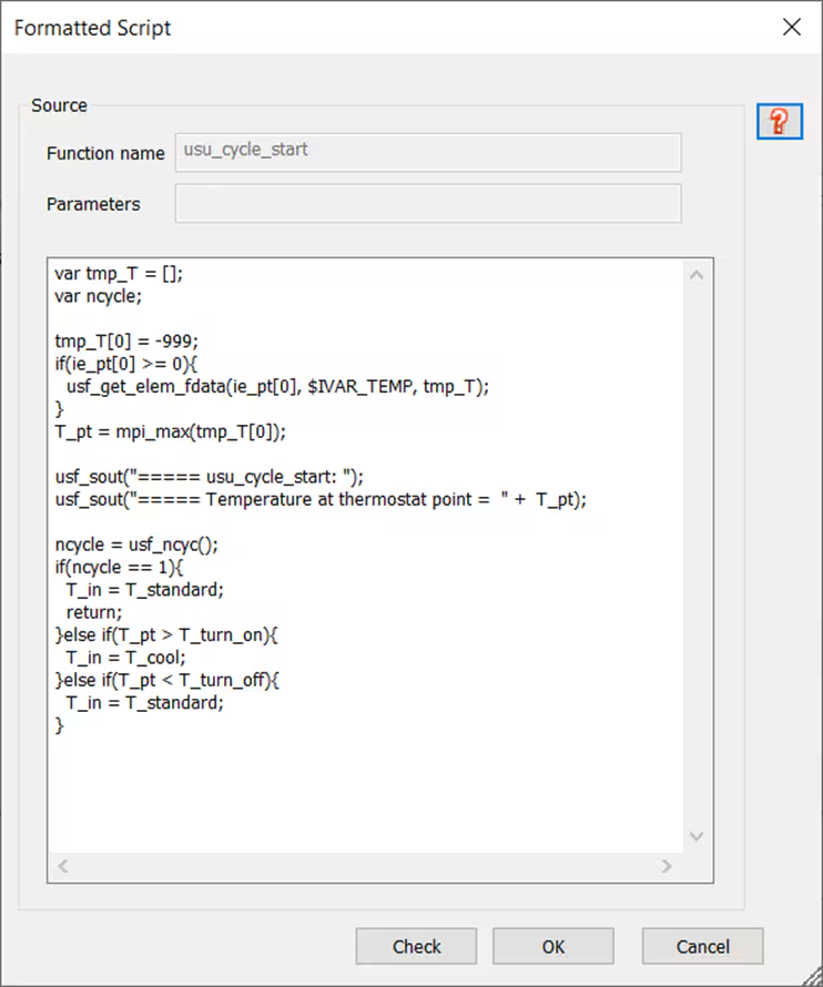
Explanation: This block executes every simulation cycle. It reads the latest monitor temperature and applies logic to switch the supply temperature between standard and cooled values accordingly.

---

✅ Final Steps

• Confirm script settings under [Script List]
• Apply and save all changes
• Run the transient solver

Once completed, visualize the results in L-File Viewer to validate thermostat operation:

• Graph temperature at the monitoring point
• Graph average temperature at [Supply]

---

💡 Summary

With only a few lines of code, scFLOW enables powerful simulation of HVAC thermostat logic. This control system improves realism and enables scenario testing for smart building applications. Whether you’re designing for comfort or energy efficiency, this technique adds flexibility and automation to your simulation workflow.

🔗 References

• Hexagon SimCompanion. “scFLOW Script Sample for Thermostatic Control of Air Supply.” Accessed June 6, 2025. https://simcompanion.hexagon.com/customers/s/article/scFLOW-script-sample-for-thermostatic-control-of-air-supply